Poisson Probability Calculator
The Poisson distribution is usually employed for modeling systems where the probability of an event occurring is low, but the number of opportunities for such occurrence is high. Reason.
Example: During the V-1 attacks on London, rumors spread that certain points were being precisely targeted. Given the poor accuracy of the V-1, this seemed unlikely, but to test the assertion, R. D. Clarke divided an area of South London into 576 sections of ¼ square kilometer each. The total number of hits in the area was 537 -- 0.932291667 per section. Clarke then used the Poisson distribution to calculate how many sections could expect 0, 1, 2, 3, 4, or 5 or more hits, if the V-1's were striking at random throughout the area. The numbers very closely matched the actual distribution, suggesting that the observed hit clusters resulted by chance. Click here to replicate Clarke's results using this calculator. Click here to see Clarke's article. (For a comparison of Clarke's results to binomial results, see Notes section below.)
Example: The celebrated Motel Carswell forfeiture case gives another example. In that case, U.S. District Attorney Carmen Ortiz brought a civil forfeiture action against a motel that had 15 drug-related incidents in a 14-year period. Given that there are ~50,000 hotels and motels in the United States, assuming a 15-year interval and an average of one incident per hotel every three years (m=5 for the 15-year period), we would expect, with 50,000 hotels and motels ("Population"), 24 would have 14 incidents, 8 would have 15, 2 would have 16, and 1 would have 17. Click here to compute the probabilities. A federal magistrate wisely dismissed the case, but only because a nearby Walmart had a similar number of drug offenses. A better reason might have been to reject the prosecution's argument as just another airhead example of the "Law of Averages" fallacy.
Example: Assume 10,000 office buildings, each building having 100 workers, and each worker having a 1/100 chance of developing nostril spasms in a given year. How many buildings will have no cases at all in a given year? And how many will have six cases? Enter 1 in the "m (Intensity of Process)" box and 10,000 in the "Number of Observations" box. Then click the COMPUTE button. The answer is that 3,679 building will have no cases at all, and five buildings will have six cases. Human nature being what it is, people will conclude that there must be something wrong with these five buildings, and seize on some unusual characteristic -- proximity to a power line, presence of mold, or some other such nonsense -- as an explanation.
Caveat arithemeticus: Please note that numbers displayed in the result table show 10 significant digits and scale from about 10-322 to 10322. Display ends when (1) cumulative probability toPrecision(10) = 1.000000000; or (2) x = 1,000; or (3) one or more factors goes out of range. If a factor goes out of range, a message is displayed showing the factor and its JavaScript value. When that occurs, note that a JavaScript value of zero or "infinity" does not really mean zero or infinity, just a positive number smaller or larger than the range of JavaScript's floating point representation. Charting is done with the Highcharts JavaScript library, which we highly recommend (click the hamburger icon on a chart for print, image or pdf download options).
Also, please note this calculator can be invoked with a querystring, specifying m and n, for example http://anesi.com/poisson.htm?m=.932291667&n=576. When the calculator is run with user input, the URL in the address bar is updated with a querystring. This is done as a convenience for the user, who may wish to save or forward a URL that will duplicate the results shown, but also to ensure that the URL matches page content. Clicking the Clear button will clear the querystring to give the bare URL.
Finally, the "n (Number of Observations)" has, of course, nothing to do with the computation of the Poisson probabilities, which are fully determined by the intensity parameter m. It is included as a convenience for computing expected values, as in the examples. If you don't care about the calculator doing this arithmetic for you, just set it to 1, and the expected values will redundantly equal the computed probabilities.
Notes
V-1 Example. While Clarke used the Poisson distribution, he could as well have used the binomial. A binomial distribution with a mean of 0.932291667 and N of 576 would have a p of 0.932291667 / 576 = 0.001618562. This is a pretty small p value, and given that the N is rather large at 576, the binomial probabilities should (for reasons given in Derivation of the Poisson Function from the Binomial below) fairly closely approximate the Poisson. And indeed they do. If you run the binomial calculator on this site with that n and p, https://anesi.com/binomial.htm?p=.001618562&n=576, the binomial and Poisson results are quite close:
| Occurrences | Binomial probability |
Poisson Probability |
|---|---|---|
| 0 | 0.3933533298 | 0.3936505599 |
| 1 | 0.3673145706 | 0.3669971367 |
| 2 | 0.1712020053 | 0.1710741862 |
| 3 | 0.05310462263 | 0.05316367941 |
| 4 | 0.01233274636 | 0.01239101382 |
| 5 | 0.002287276490 | 0.002310407787 |
Of course, the distribution observed by Clarke could have been produced if the Germans had very precise targeting capabilities and intentionally threw extra V-1's at marginal sectors to give the impression of a random distribution. That was not the case, but it is worth observing that devious adversaries can do things like that (to conceal the true accuracy potential of a weapon, for example).
Motel Carswell Case. Is it reasonable to expect that a motel in a high-crime area will have more drug deals than a motel in a low-crime area? Possibly. Or perhaps police scrutiny in high crime areas is more stringent, so more deals are detected there, even though more deals occur at the motel in a low-crime area. It's an interesting question. But clearly, estimating the frequence of an offense from the frequency of arrests or prosecutions is silly, leading to absurd conclusions -- for example, that littering is rare in rural areas because it is seldom prosecuted there, that adultery is rare in states where it is illegal because it is seldom prosecuted, or that illegal voting is rare because it is seldom prosecuted (who would make the complaint?). A cottage industry deals with questions like this, usually using half-buttocked, misspecified models with deficient data, omitted variable bias, ecological fallacies, and a ton of heroic assumptions, bizarrely passed off as establishing causal relationships.
And man, we won't even mention the idiotic bivariate charts the folks at Vox, Slate, NYT, WaPo and the Daily Kos try to pass off as implying causality. They might as well pull them from http://tylervigen.com/spurious-correlations. But we digress. The real point is that in a case like this, the first question we should ask is, "What reason do you have to believe that this departure from population means does not result from chance? If you flip a coin ten times, are you really stupid enough to be amazed if you don't get 5 heads?"
Nostril Spasms. Same observations as for the Motel Carswell Case. The occurrence of many nostril spasms in one building might result from some causative agent linked to the building, but assuming that many nostril spasms in one building imply a causative agent linked to the building is nonsense.
Derivation of the Poisson Function from the Binomial (by William L. Hays)
"Although Poisson variables and the processes generating them can be given a variety of useful interpretations, perhaps the simplest approach to the study of the Poisson is to regard it as a special case of the binomial. A derivation of the Poisson function from the binomial will now be sketched out. What we are going to show is that if N is allowed to become extremely large while p is made extremely small, and if Np remains constant, the binomial distribution approaches the Poisson distribution. Take note, however, that this is just a sketch of the general outline of a proof. A number of the mathematical qualifications really necessary to such a proof will be omitted here.
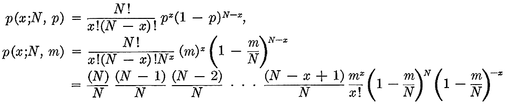
"Consider a binomial variable X, which takes on values with probabilities depending on p, the probability of success, and N, the number of trials. Let us define m = Np. Then we can rewrite the binomial probability that X = x as
 "Now we want to find the limiting value of this probability as N becomes indefinitely large and m remains constant. That is, we want to find
 "We can do so by examining what happens to the various terms in the expression
above as N approaches the limit. First of all, as N is made indefinitely large,
1 − (1/N) approaches 1, 1 − (2/N) approaches 1, and so do all of the succeeding
terms up through 1 − (x + 1)/N. The expression [1 − (m/N)]−x must also approach 1.
The only other term involving N is [1 − (m/N)]N. In the advanced
calculus it is shown that
"We can do so by examining what happens to the various terms in the expression
above as N approaches the limit. First of all, as N is made indefinitely large,
1 − (1/N) approaches 1, 1 − (2/N) approaches 1, and so do all of the succeeding
terms up through 1 − (x + 1)/N. The expression [1 − (m/N)]−x must also approach 1.
The only other term involving N is [1 − (m/N)]N. In the advanced
calculus it is shown that

"Hence, making these substitutions, we have

"For fixed m = Np, and as N becomes indefinitely large, the limiting value of the binomial probability p(x;N, m) is the Poisson probability (e−mmx)/x!.
"Because of this connection between binomial and Poisson probabilities, Poisson sampling can be thought of as the act of making a vast number of trials from a stable and independent Bernoulli process for which the probability of a success is extremely small. The constant m is called the "intensity" of the Poisson process.
"Not only does this connection with the binomial distribution permit one interpretation of the Poisson distribution; there are practical consequences as well. In cases in which N is large and p is relatively small, the binomial probabilities may be very laborious to calculate. In this instance, it is a much simpler matter to approximate the exact binomial probabilities through use of Poisson probabilities for the various values of x.
"When a Poisson probability for some specific x value is desired, one simply calculates m = Np, and then applies the Poisson rule

for the value X = x of interest."